Exploring Depth and Width in Multi-Layer Perceptrons for Credit Risk Prediction
Name: Cynthia Chinenye Udoye
Student No: 22029346
Abstract
This tutorial explores how the architecture of Multi-Layer Perceptrons (MLPs), specifically their depth (number of layers) and width (number of neurons per layer), impacts their performance in predicting credit risk. Using the "Credit-G" dataset, we address class imbalance by applying class weights and test various combinations of layers and neurons. Our findings reveal that while increasing the depth of MLPs enhances their learning capacity, it also increases the risk of overfitting. Similarly, adding more neurons often increases computational time without consistently improving accuracy. The best-performing model achieved an AUC-ROC score of 0.80. This tutorial provides a clear and practical guide for using neural networks to tackle imbalanced data challenges in credit risk prediction.
Introduction
Predicting credit risk is very important in finance. It helps banks and other financial institutions figure out which applicants are likely to repay loans, reducing the risk of losing money and increasing profits (Thomas et al., 2002). Credit risk models make the decision-making process in lending more reliable.
In this tutorial, we explore the use of Multi-Layer Perceptrons (MLPs), a type of neural network, for classifying credit data into 'good' and 'bad' risk categories. MLPs are particularly well-suited for this task due to their ability to model complex nonlinear relationships in data (LeCun et al., 2015). However, datasets like the "Credit-G" dataset often exhibit class imbalance, with significantly more 'good' cases than 'bad' (He and Garcia, 2009). To address this, we apply class weights to ensure equitable learning from both classes.
The objective of this tutorial is to investigate how the architecture of MLPs, specifically the number of layers (depth) and neurons per layer (width), influences model performance. While deeper networks can capture intricate patterns and wider layers enhance representational power, both architectures pose challenges, including increased computational cost and potential overfitting (Hinton et al., 2012). Performance will be assessed using metrics such as AUC-ROC, accuracy, precision, recall, F1-score, and validation loss, providing a comprehensive evaluation of these trade-offs.
This tutorial will take you through every step of the process, including understanding the dataset, preparing the data, testing different MLP designs, and looking at the results. By the end, we hope to gain valuable insights into building effective neural networks for credit risk prediction and similar challenges in finance.
Dataset and Preprocessing
The "Credit-G" dataset from OpenML contains financial records labelled as 'good' or 'bad' credit risks. It is commonly used in credit risk modelling because it reflects real-world lending data. However, the dataset is imbalanced, with more 'good' cases than 'bad,' making it harder for models to learn from the minority class.
The dataset includes both categorical and numerical features. The following preprocessing steps were applied:
One-Hot Encoding: Categorical features were converted into numerical values to make them usable by the model.
Scaling: Numerical features were standardised using StandardScaler to ensure that no single feature dominated the learning process.
Data Splitting: The dataset was divided into training, validation, and test sets using stratified sampling to maintain the class distribution across all subsets.
Class Weights: Class weights were calculated and applied during training to give equal importance to 'good' and 'bad' cases.
Key Considerations:
Reproducibility was ensured by using consistent random seeds for data splitting and preprocessing. Ethical considerations, such as avoiding bias amplification, were kept in mind to ensure fair treatment of both classes in the dataset.
Model Architecture and Design
The Multi-Layer Perceptrons (MLP) is a neural network that learns patterns in data. In this tutorial, the MLP was used to classify credit risks as 'good' or 'bad' based on the features of the "Credit-G" dataset (OpenML, n.d.).
1. Model Overview
Input Layer: Receives the processed dataset, with the number of input nodes equal to the total number of features.
Hidden Layers:
Multiple hidden layers were tested, varying in the number of layers (depth) and neurons per layer (width).
Each layer uses the ReLU (Rectified Linear Unit) activation function to identify complex patterns (LeCun et al., 2015).
Output Layer: Contains one neuron with a sigmoid activation function, predicting the probability of a record being a 'bad' credit risk.
Figure 1: The structure of Multi-Layer Perceptrons (MLP) consists of interconnected layers facilitating complex computations (Datacamp, n.d.).
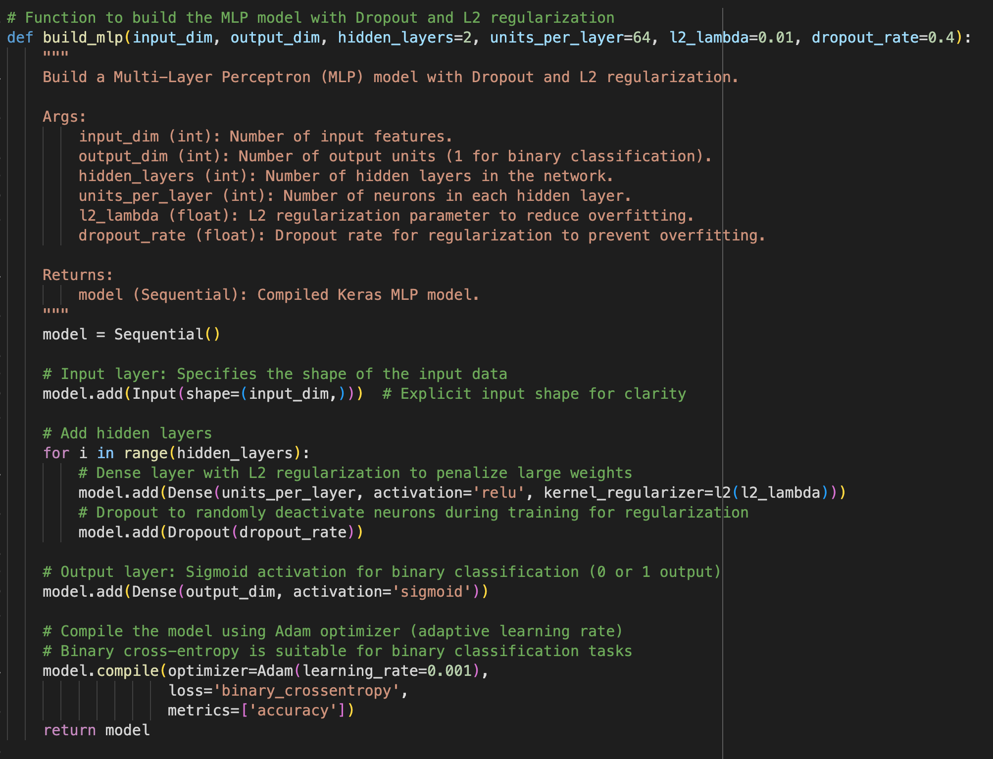
2. Building the MLP
The build_mlp_model() function creates a multi-layer perceptron (MLP) model using TensorFlow and Keras. It accepts parameters for the number of layers, neurons per layer, activation functions, and optimizer settings. The model is compiled for binary classification with metrics like accuracy and AUC. This design allows flexibility in architecture exploration, enabling customisation of depth and width to optimise performance on the dataset.
Figure 2: Building the MLP
3. Training and Evaluation with Class Weights
The train_and_evaluate_with_class_weights function trains and evaluates the MLP model while addressing class imbalance by applying class weights. It takes the model, training and validation datasets, class weights, and training parameters such as epochs and batch size. The function outputs the training history and evaluation metrics, including accuracy and AUC, to measure the model's performance effectively.
4. Experimentation and Hyperparameter Tuning
The run_experiments function automates the process of exploring various configurations of the MLP model. It iterates through combinations of depth (number of layers), width (neurons per layer), and other hyperparameters. The results of each configuration are logged to facilitate comparison and identify the optimal architecture for the dataset. This function simplifies architecture exploration and supports effective model optimisation.
5. Improving the Model
Dropout: Randomly disables some neurons during training to prevent the model from relying too heavily on specific patterns (Srivastava et al., 2014).
L2 Regularisation: Adds a penalty for large weights, helping reduce overfitting and improve the model's ability to generalise to new data (Hinton et al., 2012).
6. Impact of Depth and Width
Depth (Layers): Adding more layers helps the model learn more detailed patterns but can lead to overfitting and slower training if overdone.
Width (Neurons per Layer): Increasing neurons gives the model more capacity to learn but also increases training time without always improving performance.
Optimal Design: Tests showed that a model with 4 layers and 64 neurons per layer achieved the best trade-off between performance and complexity (Goodfellow et al., 2016).
7. Using Class Weights
The "Credit-G" dataset is imbalanced, with more 'good' cases than 'bad.' Class weights were applied to make the model focus more on the minority class ('bad'). This improved the recall for 'bad' cases, balancing the model’s predictions (He & Garcia, 2009).
Experimentation and Results
1. Experimental Setup
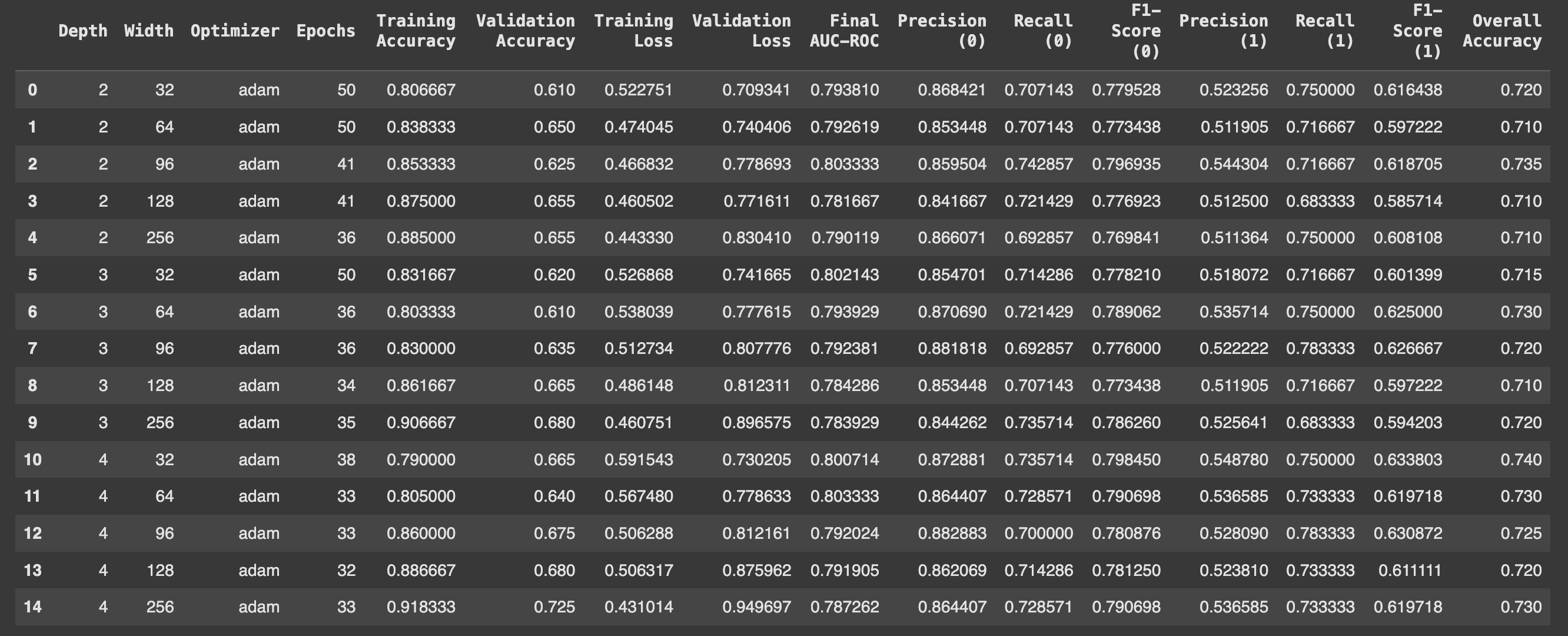
To explore how the architecture of Multi-Layer Perceptrons (MLPs) impacts credit risk prediction, different combinations of depths (number of hidden layers) and widths (number of neurons per layer) were examined. This table represents the performance of the models with varying configurations of depth, width, and epochs, using the Adam optimiser.
Depth & Width Impact: Increasing depth and width improves training accuracy but can cause overfitting, shown by higher validation loss.
Performance Trade-offs: Wider models (256) achieve better validation accuracy, converge faster, but may not always maximise AUC-ROC.
Figure 3: Impact of Depth and Width on Model Performance Metrics.
The following metrics were used to evaluate model performance:
AUC-ROC: Measures the model's ability to distinguish between 'good' and 'bad' credit risks.
Precision: Indicates how many of the predicted 'bad' cases were correct.
Recall: Measures how well the model identifies 'bad' credit cases.
F1-Score: Balances precision and recall.
Validation Accuracy: Reflects the overall correctness on the validation set.
Class weights were applied during training to handle the dataset's imbalance, ensuring both classes were equally represented in the learning process.
2. Presentation of Results
The results are summarised using heatmaps and line plots to show how performance changes with different depths and widths:
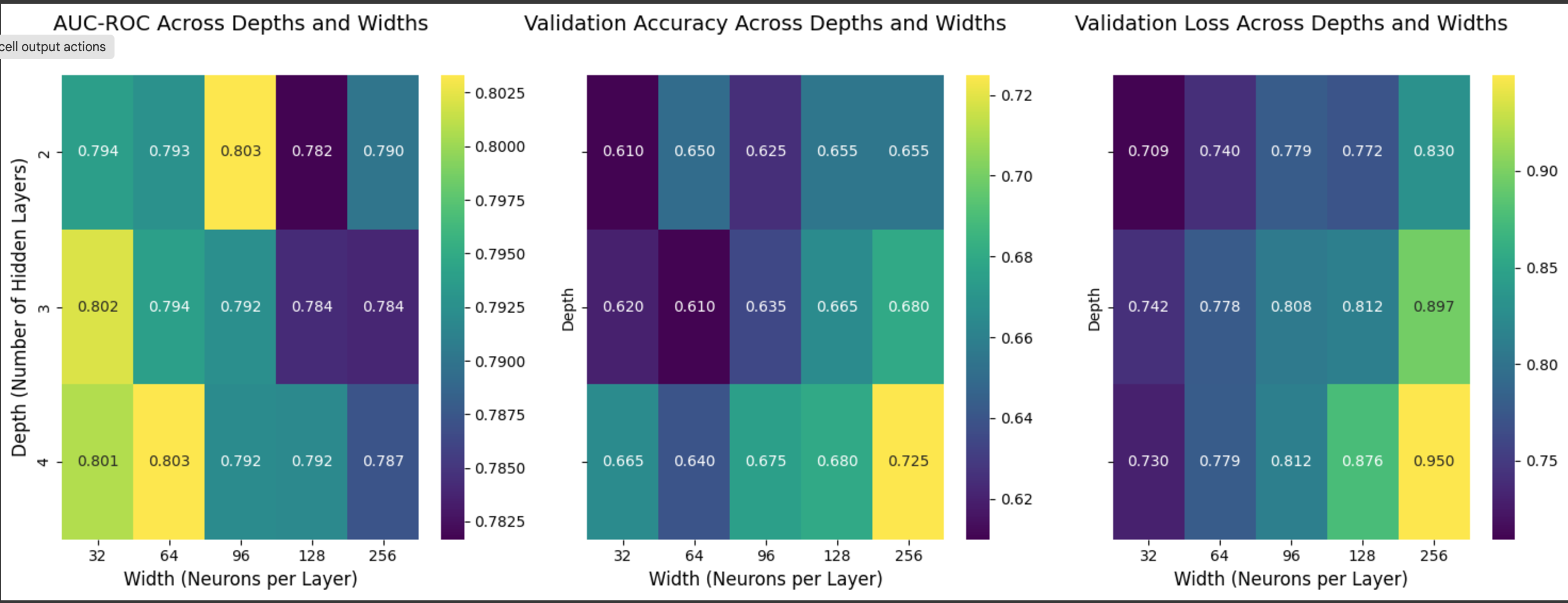
Heatmaps:
AUC-ROC, validation accuracy, and validation loss scores for all tested configurations were visualised. The best-performing model had 4 layers and 64 neurons per layer, achieving an AUC-ROC score of 0.80 and a validation accuracy of 75%.
Figure 4: Model Performance Across Depths and Widths.
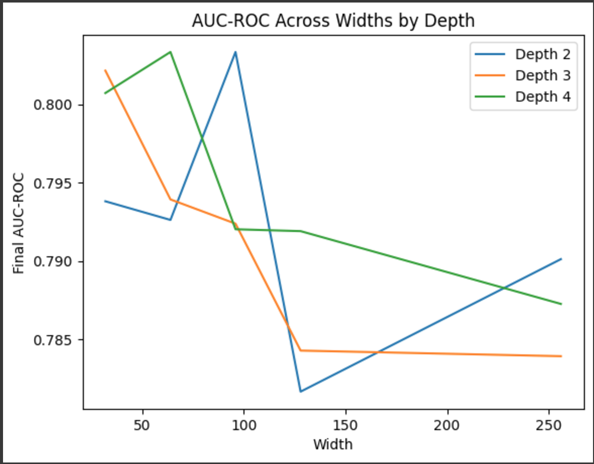
Line Plots:
Trends in AUC-ROC scores across widths for each depth showed that increasing the width generally improved performance up to a certain point (64 neurons) but slightly dropped beyond that.
Figure 5: AUC-ROC Trends Across Widths and Depths.
3. Key Observations
Impact of Depth: Adding more layers improved the model’s ability to capture patterns, but too many layers (more than 4) could lead to overfitting.
Impact of Width: Wider layers (up to 64 neurons) enhanced learning capacity, but widths beyond this provided diminishing returns.
Discussion & Evaluation of the Best-Performing Model
The best-performing model used 4 layers and 64 neurons per layer. This setup balanced learning complex patterns and avoiding overfitting or unnecessary computational cost. It effectively predicted both "good" and "bad" credit risks, even with an imbalanced dataset.
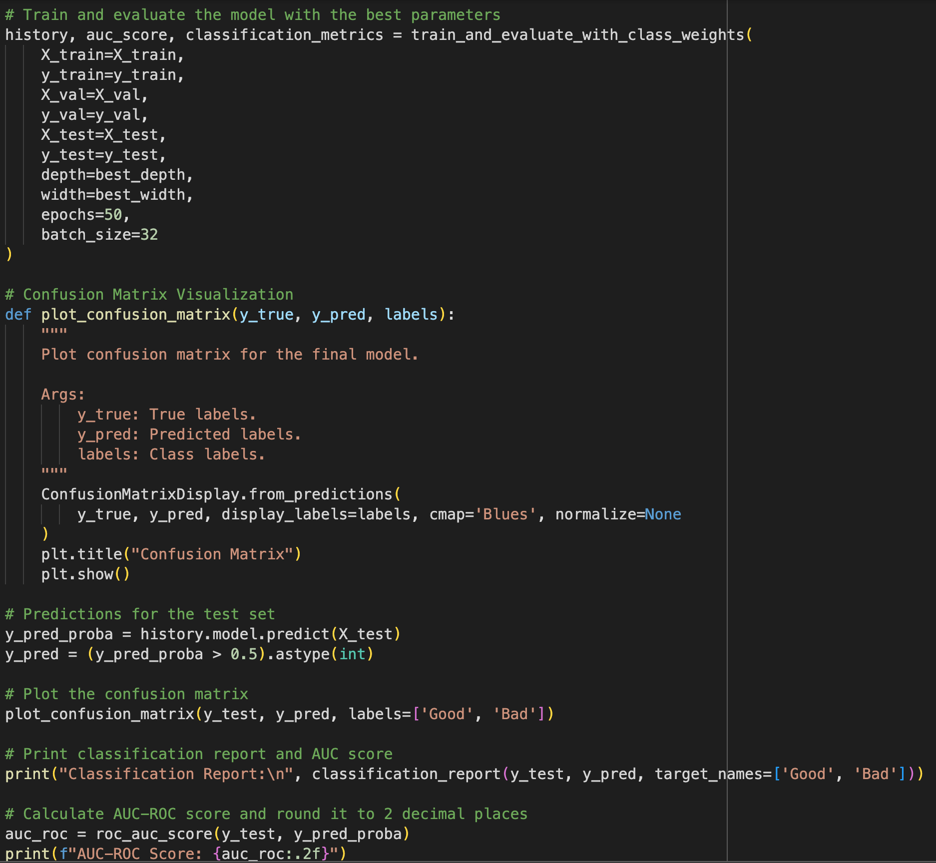
Figure 6: Model for the best depth and width.
1. Key Metrics on the Test Dataset
Precision (Good): 0.87
Recall (Good): 0.76
F1-Score (Good): 0.81
Precision (Bad): 0.56
Recall (Bad): 0.73
F1-Score (Bad): 0.64
Overall Accuracy: 75%
AUC-ROC: 0.80
This model captured complex patterns in the data while avoiding overfitting, thanks to dropout and regularization techniques. The use of class weights addressed the imbalanced dataset, ensuring that "bad" credit risks were not ignored.
While the precision for 'bad' cases was lower, indicating some false positives, the high recall ensured the model successfully identified 'bad' credit risks. This balance makes the model highly useful in scenarios where identifying risky credit cases is more critical than avoiding occasional false alarms.
By balancing depth, width, and regularization, this architecture demonstrated strong performance and reliability for credit risk prediction.
2. Confusion Matrix
The confusion matrix for the best model shows:
True Positives (Bad predicted as Bad): High recall for 'bad' credit indicates the model’s effectiveness in identifying these cases.
True Negatives (Good predicted as Good): Strong precision for 'good' credit highlights its reliability in identifying trustworthy applicants.
3. Visualisation
The confusion matrix confirms that while the model performs well overall, it still occasionally misclassifies 'bad' credit as 'good.' This misclassification may be influenced by the inherent imbalance in the dataset. However, the application of class weights during training helps mitigate this issue by emphasising the minority class, thereby balancing the trade-off between precision and recall.
Figure 7: Confusion Matrix for Model Performance Evaluation (Best Layer and Neurons Configuration).
4. Insights
AUC-ROC:
An AUC-ROC score of 0.80 indicates the model can reliably distinguish between 'good' and 'bad' credit risks. This metric reflects the model’s ability to handle imbalanced data effectively.
Precision-Recall Trade-Off:
The model’s precision for 'bad' credit (56%) is lower than its recall (73%), meaning it is more likely to catch potential bad credit cases but at the cost of some false positives.
Class Weights:
The use of class weights during training played a key role in ensuring the minority class ('bad') was not overlooked, improving its recall significantly.
Conclusion and Recommendations
This tutorial explored how the architecture of Multi-Layer Perceptrons (MLPs), specifically the number of layers (depth) and neurons per layer (width), affects their performance in predicting credit risk. The best model, with 4 layers and 64 neurons per layer, achieved a good balance between complexity and accuracy. It handled class imbalance effectively using class weights and achieved an AUC-ROC score of 0.80, along with strong precision and recall for both 'good' and 'bad' credit risks.
Practical Applications
The findings demonstrate that MLPs can be a valuable tool for credit risk prediction, helping financial institutions assess loan applications more reliably. By identifying patterns in credit data, these models can reduce default risks and improve decision-making in lending processes.
Recommendations for Future Exploration
Testing on Additional Datasets: Applying the model to other credit datasets could validate its generalisability and robustness.
Hyperparameter Tuning: Further tuning of learning rates, batch sizes, and regularisation parameters could optimise performance.
Feature Engineering: Incorporating domain-specific knowledge to create new features might improve prediction accuracy.
In conclusion, this tutorial highlights how thoughtful design choices in neural network architecture can lead to efficient and reliable credit risk models. Future work could extend these insights to other financial applications, offering even broader benefits.
Dua, D. & Graff, C., 2019. UCI Machine Learning Repository. Irvine, CA: University of California, School of Information and Computer Science.
Available at:
https://www.openml.org/d/31
[Accessed 9 Dec. 2024].
Goodfellow, I., Bengio, Y. & Courville, A., 2016. Deep Learning. Cambridge, MA: MIT Press.
Available at:
https://www.deeplearningbook.org
[Accessed 9 Dec. 2024].
He, H. & Garcia, E.A., 2009. Learning from Imbalanced Data. IEEE Transactions on Knowledge and Data Engineering, 21(9), pp.1263–1284.
Available at:
https://doi.org/10.1109/TKDE.2008.239
.
Hinton, G., Srivastava, N. & Krizhevsky, A., 2012. Improving Neural Networks by Preventing Co-Adaptation of Feature Detectors.
arXiv preprint, arXiv:1207.0580.
Available at:
https://arxiv.org/abs/1207.0580
.
Srivastava, N., Hinton, G., Krizhevsky, A., Sutskever, I. & Salakhutdinov, R., 2014. Dropout: A Simple Way to Prevent Neural Networks from Overfitting.
Journal of Machine Learning Research, 15(1), pp.1929–1958.
Available at:
http://jmlr.org/papers/v15/srivastava14a.html
.
%20consists%20of%20interconnected%20layers%20facilitating%20complex%20computations%20(Datacamp%2C%20n.d.)..png)
.png)